
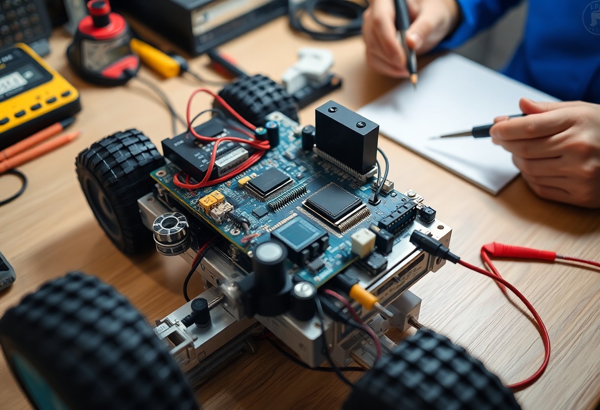
Over a dozen sensor options shape your design choices; you must weigh range, resolution, and interface compatibility. This post outlines selection, integration, and testing so you can build an effective sensing system for a custom robot.
Sensor Selection and Requirement Analysis
Choose sensors that match the measurements you need, interface with your controller, fit your power budget, and meet cost targets; prototype selections early to validate real-world performance.
Defining Operational Constraints and Environment
Assess environmental factors like temperature, lighting, EMI, and physical obstructions so you can pick sensors with appropriate enclosures, ranges, and mounting options.
Accuracy, Resolution, and Sampling Frequency
Balance accuracy, resolution, and sampling rate against processing and data bandwidth to ensure measurements are actionable without overloading your system.
Detailed evaluation should have you examine sensor noise, linearity, hysteresis, and temporal response. You must calculate required resolution from expected signal variation, derive sampling frequency from Nyquist and system dynamics, and budget processing time for filtering. Practical tests under operational conditions will reveal if your chosen specs meet control and perception needs.
Navigation and Spatial Perception Hardware
Sensors you choose determine spatial awareness; combine LiDAR, ultrasonic and IMUs, and consult How to Make a Robot – Lesson 7: Using Sensors for practical setup and wiring tips.
LiDAR and Ultrasonic Ranging Systems
LiDAR provides dense 2D/3D scans for mapping and obstacle detection while ultrasonic sensors offer low-cost short-range checks, so you should match placement and update rates to task requirements.
Inertial Measurement Units and Odometry Integration
Inertial Measurement Units fused with wheel odometry smooth pose estimates during short sensor dropouts, and you should calibrate gyros, correct encoder bias, and tune your filter to limit drift.
Fusion of IMU and odometry requires modeling sensor noise and bias in an EKF or complementary filter; you must detect wheel slip with consistency checks, apply gyro bias calibration, and inject periodic absolute fixes from visual odometry, GPS, or LiDAR loop closures to bound long-term drift and simplify tuning.
Visual Systems and Depth Perception
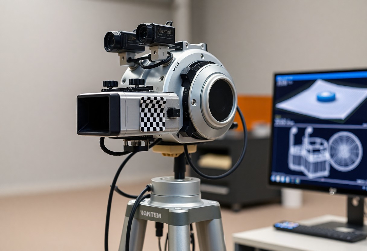
Depth perception ties stereo cameras, ToF sensors, and structured-light modules so you can build accurate 3D maps for obstacle avoidance, grasp planning, and SLAM.
Stereo Vision and Time-of-Flight Cameras
Stereo vision offers dense depth from parallax, while time-of-flight cameras deliver direct distance readings; you should choose based on range, latency, and lighting constraints.
Real-time Feature Extraction and Tracking
Feature extraction reduces image data into points and descriptors so you can track motion, estimate pose, and trigger control loops at frame-rate.
Tracking relies on fast detectors (ORB, FAST), descriptors (BRIEF, ORB) and motion models so you can maintain consistent landmarks under motion and lighting changes. You should combine feature matching with RANSAC and a Kalman or particle filter to reject outliers and smooth pose estimates. Hardware acceleration and fixed-point optimizations reduce latency; tune feature count and descriptor size to balance accuracy and throughput on your compute budget.
Data Acquisition and Hardware Interfacing
Data acquisition ties sensors to your controller via ADCs, multiplexers, and level shifters; you must match sampling rates, resolution, and input ranges while planning channel count, grounding, and power to minimize measurement error and ensure consistent readings.
Communication Protocols: I2C, SPI, and CAN Bus
I2C, SPI, and CAN present tradeoffs in speed, topology, and noise tolerance; you should choose I2C for simple sensor networks, SPI for high-speed point-to-point links, and CAN for longer, noisy runs requiring multi-node arbitration and error handling.
Signal Conditioning and Electromagnetic Interference Mitigation
Shielding, proper grounding, and input filtering reduce EMI before conversion; you must use twisted pairs, differential signaling, ferrites, and decoupling placement to lower noise and protect ADC accuracy on sensor inputs.
You should design input stages with impedance matching, RC low-pass filters, and common-mode chokes to reject high-frequency noise. Use differential ADC inputs or instrumentation amplifiers for small signals, add series resistors and TVS diodes for surge protection, and keep analog and digital grounds separated with a single-point star near the ADC. Pay attention to short analog traces, strategic decoupling, cable shield termination, and ferrite beads to maintain clean measurements.
Sensor Fusion and State Estimation
Sensor fusion blends IMU, lidar, camera and wheel odometry so you get a consistent pose estimate; state estimation filters convert noisy measurements into actionable position, velocity, and orientation for your control and planning loops.
Implementing Kalman and Complementary Filters
Kalman filters model system dynamics and sensor noise so you can fuse predictions with measurements; complementary filters offer a lightweight alternative for attitude by combining short-term IMU with longer-term references.
Temporal Alignment and Data Synchronization
Timestamp alignment ensures measurements from different sensors share a common time base so you can correctly associate observations; you should interpolate, buffer, or use hardware sync to prevent latency-induced errors in fusion.
Careful temporal alignment requires a shared clock or precise timestamping so you can correlate samples: use hardware triggers, PPS/TSYNC or PTP for a common timebase, timestamp at the driver to avoid bus latency, and calibrate fixed delays. Apply interpolation or state buffering for late packets, represent timing jitter in the filter covariance, and monitor dropped frames to keep the estimator stable.
System Calibration and Power Optimization
Calibration cycles tune sensor biases, synchronize timestamps, and trim power budgets so you sustain measurement accuracy while extending runtime across varied operating conditions.
Cross-Sensor Calibration Procedures
Align sensors using common reference motions or fixed targets, collect synchronized samples, compute offsets and scale, and then you validate results with in-situ tests to ensure modal consistency.
Balancing Computational Latency and Power Draw
Optimize processing by batching noncritical tasks, employing duty cycles, and scaling hardware resources so you meet deadlines without unnecessary energy costs.
Managing latency-power tradeoffs requires profiling your workload to identify peak compute bursts and idle intervals. You can offload heavy perception kernels to accelerators, use dynamic voltage and frequency scaling for cores, and implement adaptive sampling so sensor rates match task urgency. Prioritize interrupts for safety-critical paths and batch less urgent processing during low-power windows, then measure latency and energy per inference to set performance budgets and graceful fallback modes under battery constraints.
Summing up
Summing up, you design sensor placement for coverage, select interfaces and sampling rates to match control loops, calibrate and test for noise and drift, and integrate filtering and safety checks so the robot performs reliably in its tasks.